LTspice Tools and Applications
Contents
LTspice Induction Motor Simulation
I have been looking at existing simulation models for induction motors and found a particularly interesting one by Sohor and Kubov that appears several places on the Internet. I used the Spectrum Software application note about this model as a starting point and, after much pain, got a working induction motor model in LTspice. However, it turns out that a working version of this model had already been created for LTspice and uploaded to our group's files section.
Going through the painful process of reinventing the wheel (or motor) was not all for naught because in doing so I got to understand how the model works. It actually is very compactly written to the point of obscuring its basic operation. I have deconstructed it into its various parts as separate function modules in order to facilitate understanding. The original SK model uses transformer coupling coefficients to implement the three phase to two phase (DQ) translation and to implicitly build the inductive T-network that represents the stator, air gap and rotor. This requires the use of negative and zero coupling coefficients, making it very difficult to understand how the model works. Also the SK model indirectly accesses flux by looking at current times inductance, which only works with ideal, linear inductances. I have separated these various functions and more directly modeled flux so that saturating inductance (LTspice's Chan model) can be used in order to model motor saturation (assuming no mistakes have been made along the way).
When an induction motor first starts, the rotor is at a standstill and the sees the full line frequency, but as it speeds up, it sees only the difference between its angular speed and the stator field rotating at the line frequency, which may be a fraction of a Hertz at full speed. This frequency shift in the rotor's frame of reference affects the penetration depth of rotor current and its effective resistance and inductance. The basic SK model does not address this effect at all, but it may be possible to add these effects to the LTspice version of the model. - a.s.
Model Here: File:Simplified 2-Phase Induction Motor (with saturation).asc
More Complete files including 3 phase motors
How to convert SPICE Netlist to an LTspice schematic
Schematic Builder to automate the first steps below.
Before you start, make working copy of the netlist and then clean it up by doing any reordering of lines or shortening of node/net names that will make them easier to work with. For example, nets with names like "n023" and "n001" can usually be safely shortened to "n23" and "n1" (sometimes I do this in a word processor with find and replace). Also, it is a good idea to move all comments to the end of the working netlist (if not delete them altogether).
At this point, I like to import the netlist into LTspice, either directly onto the schematic (if the netlist is short) or into a separate LTspice netlist window.
Now go through the netlist line by line and place a component of the corresponding type on the schematic (arrange these in rows by component type such that you build up rows of all the same type). It is important to do this in exactly the same order as the net- list because this will greatly ease cross checking when you think you have finished. (Also, all of the SPICE text, such as model statements, etc. should be copied and pasted in at the end.)
As you place each component, edit its reference designator to agree with the corresponding netlist reference designator.
As you place each component, place a net-label/node-name directly on each pin of the component (of course, these should agree with their names in the netlist, too). Don't bother with wires yet as these will just be trouble to move around later.
Once all the components are placed, view the SPICE Netlist (it's a drop-down menu item) and verify that it agrees *exactly* with the original netlist (it will, if you followed these instructions carefully). Correct any errors as needed until agreement is perfect. This "schematic" should actually be able to run at this point.
(This above section is what is automated by the SchBuilder.)
So far you have just been playing the part of a robot, but now comes the fun part where human judgement is required. Move the components around on the schematic to group them such that the pins that have the same net names are close to each other and that signal flow makes sense. Use the Highlight Net tool (right mouse button click on a pin or net) to make sure no connection is overlooked.
Only when the parts are reasonably well placed is it time to start drawing in the wires and adjust the look of the schematic.
Be sure to check occasionally that the two netlists continue to match.
Because both netlists and schematics are just ascii text files, the first part of this process should be fairly straightforward to automate in software. Grouping components and connecting them for least total wire length might be harder, but still possible (I would try an approach using the so-called "synthetic annealing" algorithm). However, finishing the schematic to human sensibilities would seem beyond the reach of any canned program, but having a utility that did the first two steps would be a big time saver and well worthwhile. (from analogspiceman, used by permission)
Source Code for Schematic Builder is available here or
as one zip file available here
You need to use Lazarus a Pascal based development tool.
After you have installed the latest version of Lazarus, double-click on SchBuilder.lpr to open the project. Further development and LTwiki updates are encouraged.
Comparing LTspice and Oscilloscope Waveforms
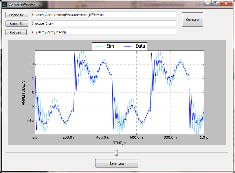
Sometimes you want to see how closely your SPICE simulation matches the real circuit as seen by your scope. Here is a utility which imports an LTspice waveform and the data from your scope, overlays them, and allows you to slide one back and forth to line them up. It’s called CompareWaveforms, and here’s what it looks like:
You select the files to compare, press Compare, and use the long slider along the bottom to line up the waveforms. You can save the plot as a .png file to include in a report.
The formats of the input files are straightforward. The LTspice file is the direct output of File / Export from the LTspice waveform window. The scope file is a .csv (Comma-Separated Values text file) with two header lines at the beginning (because that’s what my scope puts out). Each subsequent line is of the form time-in-seconds, volts. These are easily changed in the Python source if you wish. The scope data file may have a time offset due to trigger delay or trace positioning, so that is subtracted from the scope time measurements to match the LTspice time which starts at zero.
Note on waveform comparison: you may want to include the loading of your scope probe in your simulation. My probes are 12 pF in parallel with 2.2 Mohm, which can alter the simulator waveforms. Also, make your total simulation time equal to the sweep time of your scope (typically the time/div times 10), and make the start of the waveform roughly the same. CompareWaveforms allows you to adjust time +/-10% of the total sweep.
Compare Waveforms Complete Install for Windows
Compare Waveforms Python 3.4 Source Code
More info and tools at Exality
Computation of SPICE diode parameters from 3 electrical measurements
This calculator tool is a Mathematica CDF (Computable Document Format), the CDF player is a 200MB download from the Wolfram site.
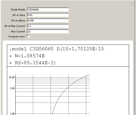
It takes 3 measurements either taken on the real device or from the datasheet to determine IS, N, Rs. This application uses the Mathematica Symbolic and numerical solvers to invert the diode current vs voltage formula.
Enter the 3 measurements in the input fields and click the checkbox "Compute now!" to get the diode definition line and the current vs voltage graph as shown in the picture below.
Actual application is below, must download and install the CDF player from Wolfram the be usable.

